You Can Find Geodesic Paths in Triangle Meshes by Just Flipping Edges
Abstract
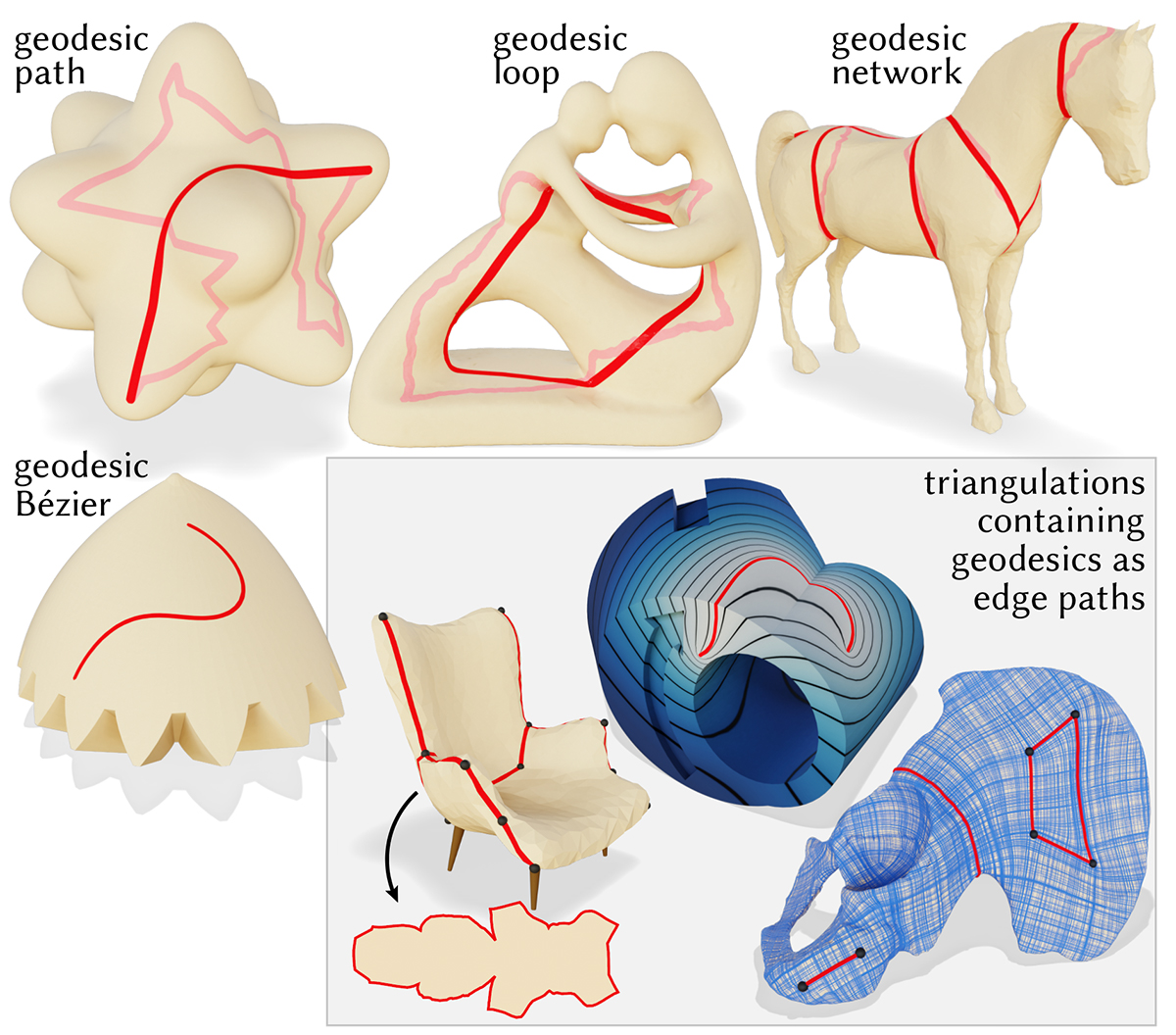
This paper introduces a new approach to computing geodesics on polyhedral surfaces—the basic idea is to iteratively perform edge flips, in the same spirit as the classic Delaunay flip algorithm. This process also produces a triangulation conforming to the output geodesics, which is immediately useful for tasks in geometry processing and numerical simulation. More precisely, our FlipOut algorithm transforms a given sequence of edges into a locally shortest geodesic while avoiding self-crossings (formally: it finds a geodesic in the same isotopy class). The algorithm is guaranteed to terminate in a finite number of operations; practical runtimes are on the order of a few milliseconds, even for meshes with millions of triangles. The same approach is easily applied to curves beyond simple paths, including closed loops, curve networks, and multiply-covered curves. We explore how the method facilitates tasks such as straightening cuts and segmentation boundaries, computing geodesic Bézier curves, extending the notion of constrained Delaunay triangulations (CDT) to curved surfaces, and providing accurate boundary conditions for partial differential equations (PDEs). Evaluation on challenging datasets such as Thingi10k indicates that the method is both robust and efficient, even for low-quality triangulations.
Selected figures
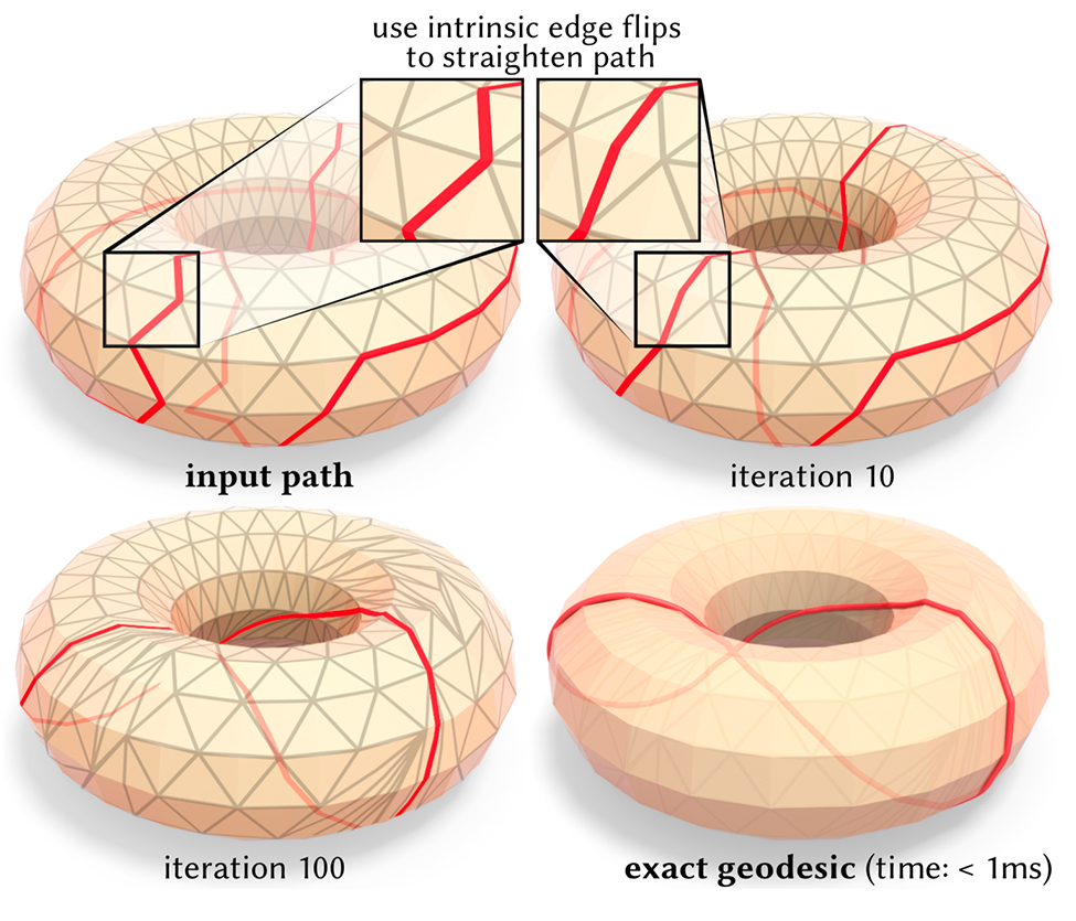
Our algorithm straightens an input edge path (top left) to an exact polyhedral geodesic (bottom right). By systematically flipping edges of an intrinsic triangulation, we provably make the curve shorter on each iteration.

FlipOut shortens a path through three consecutive vertices by pulling it as tight as possible (left, dashed line). To do so, it performs all valid edge flips in the ‘wedge’ of triangles (in blue) incident on the middle vertex i. The curve along the outside of the wedge (far right) is always shorter.
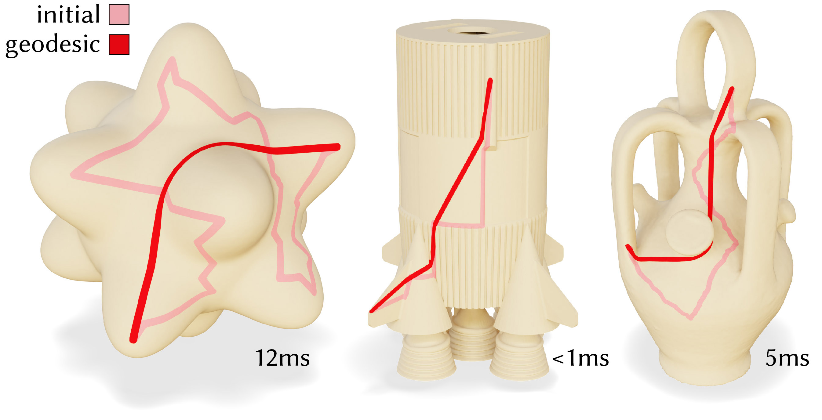
Basic results from our method, where an initial path is shortened to a geodesic by flipping edges. Inset values give the runtimes. All of the resulting curves shown are exact polyhedral geodesics.
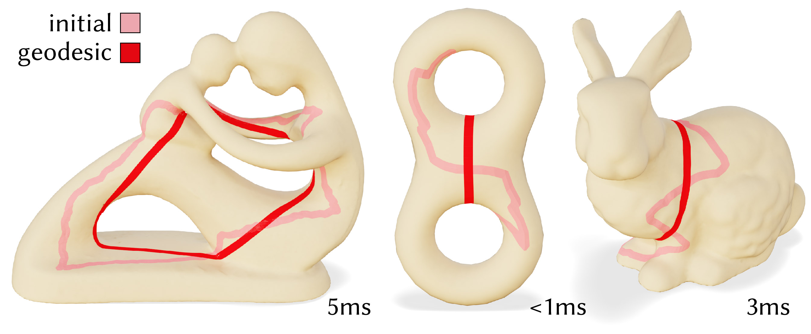
Our method also applies to loops, here an initial loop is shortened to a geodesic by flipping edges.

Independently straightening each curve can introduce new crossings, which is problematic if the curves are meant to represent region boundaries. Our flip-based approach naturally preserves the given regions.
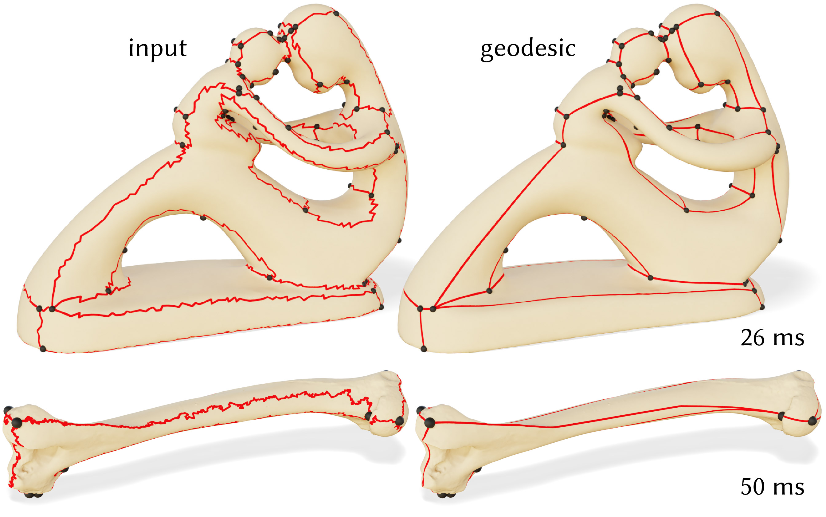
Curve networks arise naturally as texture seams in parameterizations; our algorithm can straighten these networks while preserving the cut topology. Here, seams on 3D scans of a statue (top) and a panda humerus bone (bottom) are shortened to geodesic, while preserving seam junctions.
![Meshes are often segmented by labelling faces, but the resulting regions have unintended jagged edges. Our method straightens the boundaries of these regions, yielding a more natural smooth regions while provably preserving patch topology; a length threshold prevents excessive drift. Segmentations from Chen et al. [2009].](/media/papers/flip-geodesics/segment_straighten.jpg)
Meshes are often segmented by labelling faces, but the resulting regions have unintended jagged edges. Our method straightens the boundaries of these regions, yielding a more natural smooth regions while provably preserving patch topology; a length threshold prevents excessive drift. Segmentations from Chen et al. [2009].
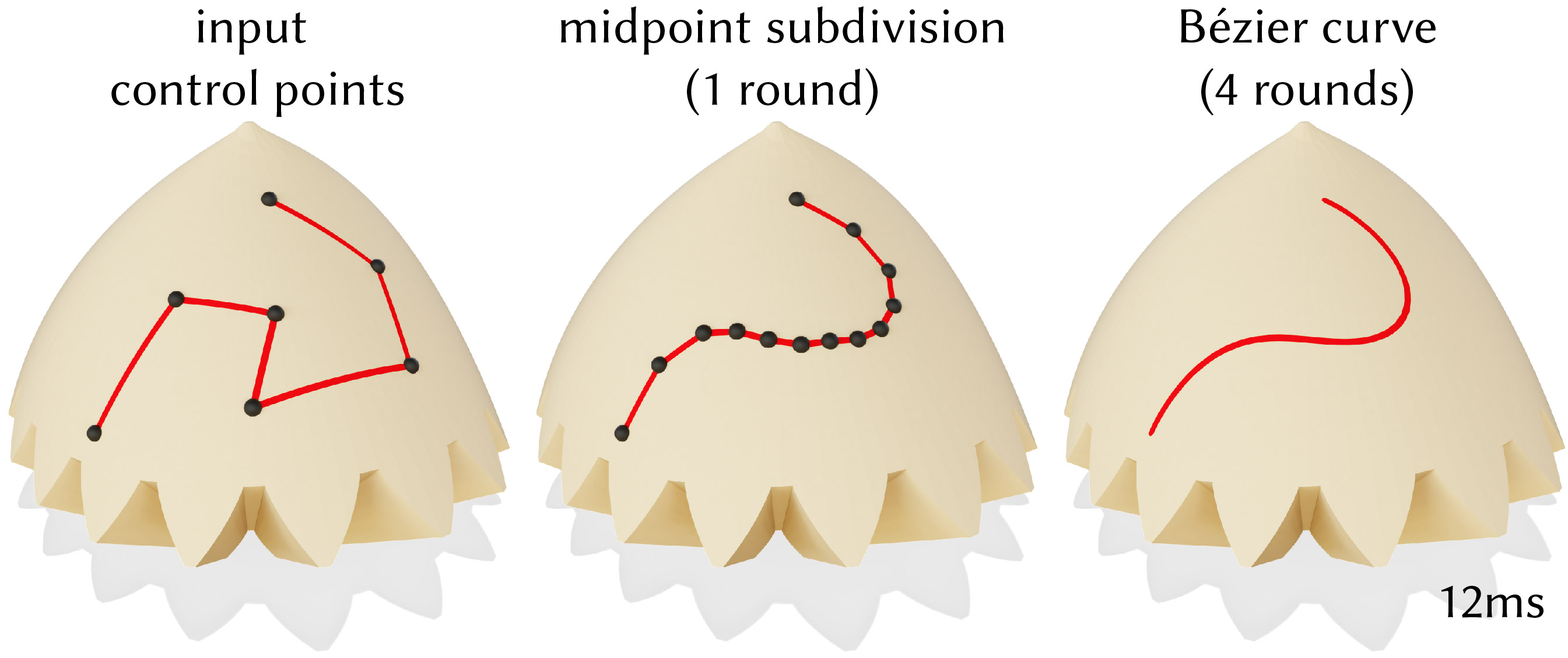
Bézier curves are widely used to represent smooth curves in space. Geodesic shortening provides the necessary operation to construct Bézier curves on surfaces, via midpoint subdivision with de Casteljau’s algorithm.
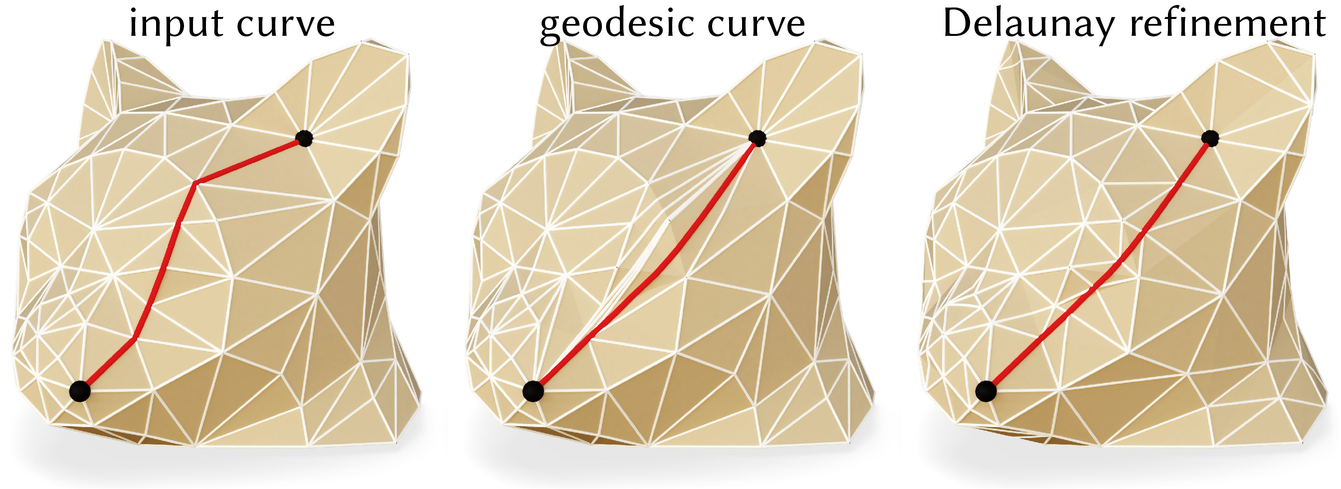
Straightening a geodesic may introduce long skinny triangles (center); applying intrinsic Delaunay refinement as a post-process yields a high quality triangulation well-suited for subsequent computation (right).
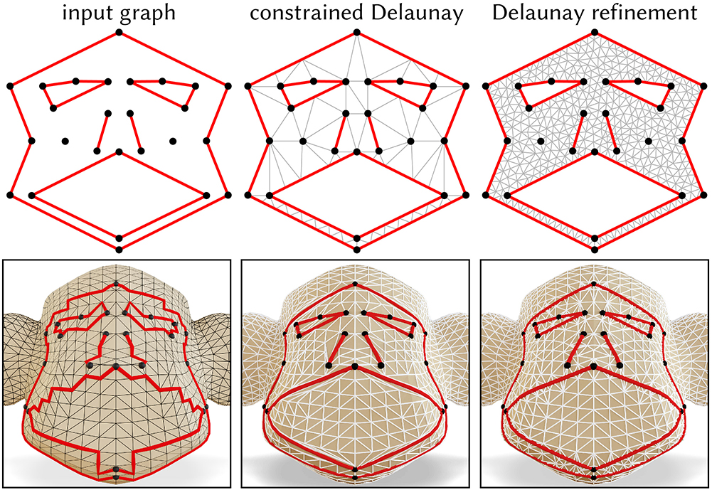
In the plane, a constrained Delaunay triangulation (CDT) (top center) contains a given set of input segments (top left); CDTs with good angle bounds (top right) are critical for, e.g., numerical simulation. The intrinsic triangulations produced by our geodesic straightening procedure extend CDTs to surface meshes (bottom row).
![Our conforming intrinsic triangulations allow geodesic or Bézier curves to be used as boundary conditions for existing algorithms. Top: a smooth cross field on a scan of a human pelvis, aligned with exact geodesic curves constructed via FlipOut. The field is generated with [Knöppel et al. 2013]. Bottom: we construct a Bézier curve on a mechanical part, then solve a Poisson problem with boundary conditions along the curve.](/media/papers/flip-geodesics/pde_examples.jpg)
Our conforming intrinsic triangulations allow geodesic or Bézier curves to be used as boundary conditions for existing algorithms. Top: a smooth cross field on a scan of a human pelvis, aligned with exact geodesic curves constructed via FlipOut. The field is generated with [Knöppel et al. 2013]. Bottom: we construct a Bézier curve on a mechanical part, then solve a Poisson problem with boundary conditions along the curve.
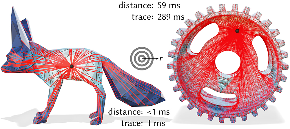
Our approach can also be used to find geodesics to all vertices from a single source. Perhaps surprisingly, all of these geodesic edges exist simultaneously in a single intrinsic triangulation.
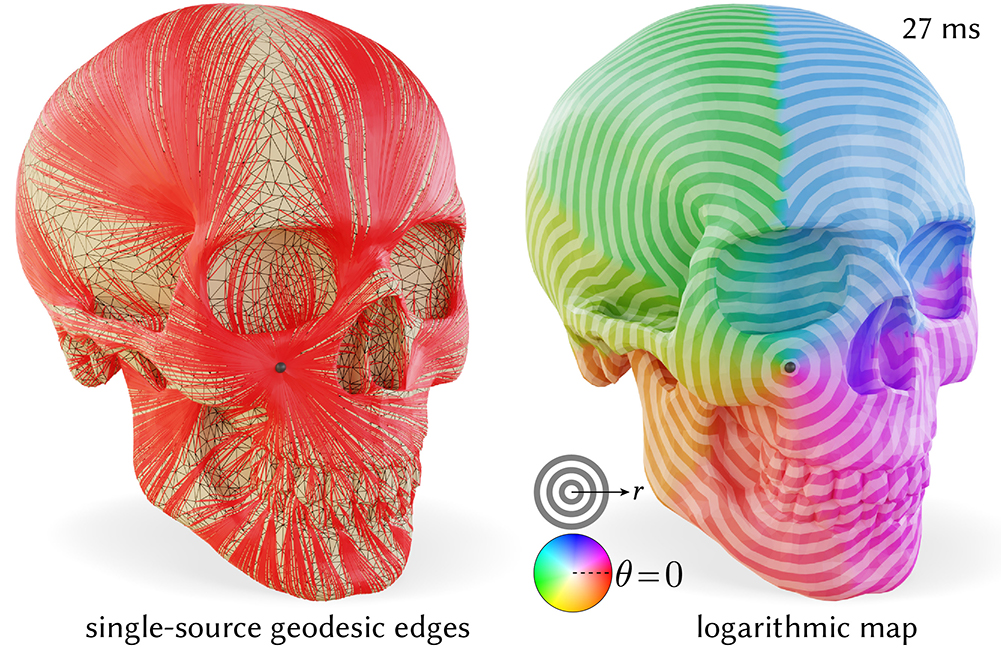
Our FlipOut procedure can be used to efficiently introduce a geodesic edge path from a single source to all other vertices (left). Reading off distance to each vertex and the direction of the edges emanating from the source yields a discretization of the logarithmic map (right). The cyclic color palette encodes the angular component of the logarithmic map, while stripes denote isocontours of its magnitude.